Motivation
Before I presented an application of Bayes Theorem in GDA. Bayes theorem can also be applied to text classification problems as well through a Naive Bayes classifier. If we were to classify a peice of text using word counts we would do so using a joint probability. We can also use the generative Bayes Classification rule to do so. At least one motivation for using Naive Bayes for this approach is that many other classifiers will fail for various reasons given such a large feature space, like the number of unique words in a given dataset. It also gives me an excuse to do something with FiveThirtyEight’s Russian troll tweet dataset.
Naive Bayes in Text Classification
Here’s that joint probability I mentioned. Assuming there are $m$ unique words in our dataset, and class labels $y$:
The big assumption is that our features are all independent from eachother with respect to the classes $y$. As in, seeing the word “shop” does not increase the likelihood of seeing the word “buy” in an email (we of course know that it would). This assumption reduces the number of parameters in the model significantly and lets us throw something together very quickly.
Ng presents the case where $Y$ takes on two values zero or one, and each $w_i$ takes on values zero or one, representing simply the presense of a word in a document which can take on only two classes. If we want more than two classes, and also if we want to take into account instances where words appear more than once, it just ends up looking a little different when we place the Likelihood function with the assumption above into Bayes rule:
In the last case I introduced a new index, $l$, for the word sums. $w_{il}$ indexes over each word, and over each count of each word. So we’ve added more terms to fit, but fitting is already pretty fast for Naive Bayes so it’s not much of a price to pay. Intuitively, I like the idea of the multinomial representation better, it allows for a “softness”, maybe a few words appear once in a piece of text by chance, but multiple occurances of some words could have far more decisive power when determining the class of the text.
As with GDA the prediction rule is then to simply assign the class with the highest probability given the Likelihood, Prior, and Evidence terms. It turns out we can actually eliminate the Evidence term, as it is constant when looking for a maximum among $Y\in[y_0 \ldots y_k]$ :
So, in order to make predictions, we just need to know all of the Prior terms $P(Y = y_k)$ and all of the Likelihood terms $P(w_m | Y = y_k)$, in either the binomial or multinomial case. The maximum likelihood estimates for each of the Likelihood terms looks like:
Or in english, the percent of cases where the class was of class $k$ and you observed your feature $w_{ij}$. Likewise the estimate for the Priors is just the percent of cases where the class of the document is of the particular class:
At this point, everything is calculable! No regressions to run, we just have to calculate all of these terms for a large enough dataset, and then attempt to make predictions with them on remaining data.
Code
There was a little bit of parsing to be done before anything could be ran; I ended up using the Natural Language Toolkit for tokenization and string cleaning, and then built in Python dicts are already hash maps which are exactly what you want when keeping and searching a large histogram of word counts. I also parsed against a set of stop words, which is common practice. Words like “A”, “an”, “or” which appear too frequently to offer much predictive quality.
	def _formCounts(self, trainingRatio):
		'''
		Helper, given the ratio of data to use for training, generate
		a dictionary of count entries ['word': count]
		@param trainingRatio		A number [0.0 : 1.0] corresponding to the fraction
									of data entries to use when building the model.
		'''
		self.numRussiaSamples = int(self.russiaData.shape[0] * trainingRatio)
		self.numNormalSamples = int(self.normalData.shape[0] * trainingRatio)
		self.totalSamples = self.numRussiaSamples + self.numNormalSamples
		self.normalDataCounts = dict()
		self.russiaDataCounts = dict()

		print("Reading in normal data counts:")
		normalErrors = 0
		for i in tqdm(range(self.numNormalSamples)):
			try:
				self._tally(self.normalData['text'][i], self.normalDataCounts)
			except TypeError:
				normalErrors += 1
		print("Failed to read " + str(normalErrors) + " lines from normal data")

		print("Reading in Russian data counts:")
		russianErrors = 0
		for i in tqdm(range(self.numRussiaSamples)):
			try:
				self._tally(self.russiaData['text'][i], self.russiaDataCounts)
			except TypeError:
				normalErrors += 1
		print("Failed to read " + str(russianErrors) + " lines from normal data")
self._tally simply increments the dict value or adds it if not present, given that the word is not in our list of stop words. Having collected word counts from each dataset (where a given tweet is only allowed to increment a count once for a given word) the calculations for Likelihood and the Prior are easy:
	def _predict(self):
		'''
		Run predictions on the data which remains after using some portion of it
		for building a model.
		@returns results: 		A named tuple with members:
								results.accuracyNormal,
								results.accuracyRussian
		'''

		# Calculate priors up front, they are constant for each prediction:
		RussianPrior = self.numRussiaSamples / self.totalSamples
		NormalPrior = self.numNormalSamples / self.totalSamples

		print("Attempting predictions on the remaining normal dataset:")
		normalNumCorrect = 0
		normalNumIncorrect = 0
		normalErrors = 0
		for idx in tqdm(range(self.numNormalSamples, self.normalData.shape[0])):
			RussianLikelihood = 1
			NormalLikelihood = 1
			try:
				for word in nltk.word_tokenize(self.normalData['text'][idx]):
					lword = word.lower()
					if(lword not in StopWords and lword not in StopPunctuation):
						RussianLikelihood *= self._laplaceLikelihood(lword, self.russiaDataCounts, self.numRussiaSamples)
						NormalLikelihood *= self._laplaceLikelihood(lword, self.normalDataCounts, self.numNormalSamples)

				RussianProb = RussianLikelihood * RussianPrior
				NormalProb = NormalLikelihood * NormalPrior
				if RussianProb > NormalProb:
					normalNumIncorrect += 1
				else:
					normalNumCorrect += 1
			except TypeError:
				normalErrors += 1

		print (str(normalErrors) + " Errors when predicting on normal data")
		accuracyNormal = (normalNumCorrect) / (normalNumCorrect + normalNumIncorrect)*100.0
		print ("Accuracy in predicting on the normal dataset: " + str(accuracyNormal))

		print("Attempting predictions on the remaining Russian dataset:")
		russianNumCorrect = 0
		russianNumIncorrect = 0
		russiaErrors = 0
		for idx in tqdm(range(self.numRussiaSamples, self.russiaData.shape[0])):
			RussianLikelihood = 1
			NormalLikelihood = 1
			try:
				for word in nltk.word_tokenize(self.russiaData['text'][idx]):
					lword = word.lower()
					if(lword not in StopWords and lword not in StopPunctuation):
						RussianLikelihood *= self._laplaceLikelihood(lword, self.russiaDataCounts, self.numRussiaSamples)
						NormalLikelihood *= self._laplaceLikelihood(lword, self.normalDataCounts, self.numNormalSamples)

				RussianProb = RussianLikelihood * RussianPrior
				NormalProb = NormalLikelihood * NormalPrior
				if RussianProb < NormalProb:
					russianNumIncorrect += 1
				else:
					russianNumCorrect += 1
			except TypeError:
				russiaErrors += 1

		print (str(russiaErrors) + " Errors when predicting on russian data")
		accuracyRussian = (russianNumCorrect) / (russianNumCorrect + russianNumIncorrect)*100.0
		print ("Accuracy in predicting on the russian dataset: " + str(accuracyRussian))

		results = namedtuple("Results", ["accuracyRussian", "accuracyNormal"])
		return results(accuracyRussian, accuracyNormal)
Results
I ran the classifier against a selection of Twitter data from FiveThirtyEight’s Russian troll tweet dataset using a more or less conversational Twitter data set from a study on geolocation data related to twittering as the baseline. Right out the gate this data isn’t all that impressive; ideally i’d like to compare the Russian dataset to a politically minded subsection of twitter during the 2016 election. Political phrases, names of politicians, and socially charged language all quickly become the strongest predictors for the Russian classification, which is cool but not all that interesting. This isn’t surprising given that my baseline is just everyday twitter, and worse yet from 2009-2010. This is due to a lack of historical data and overall access to large datasets through Twitter’s developer API; I had to use what other people had already put together.
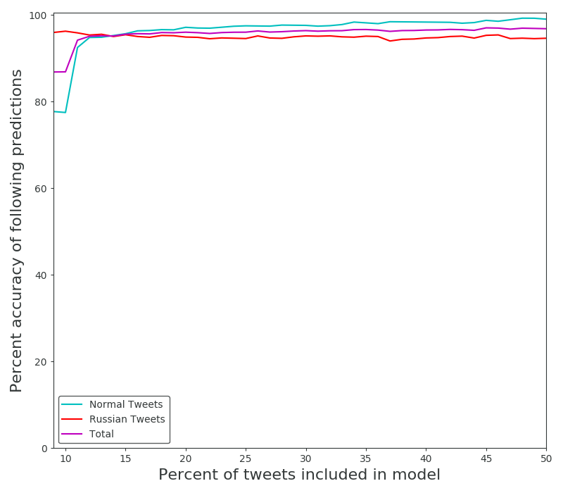
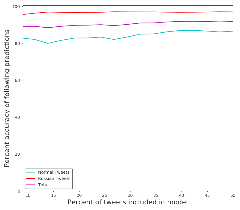
Still, the results do show off the power of Naive Bayes classification even if it is a really easy case. We can also see how the algorithm relatively struggles to classify the more difficult dataset (non-Russian) due to it’s lack of prevalent, dominating terms.

It also performs worse for larger datasets when scaling the ratio of samples used to build the model, but only for the non-Russian dataset. The Russian accuracies for these runs were 94.6, and 96.9% when using half of the data for the model, The Normal accuracies were 99, and 86.5%. It’s worth mentioning that I have not performed cross validation, these runs always took some percent of the dataset from the top to use as the model. Cross validation would smooth out the jagged behavior caused by different order of introductions with respect to certain words.

Using scikit-learn
As long as we’re learning this stuff I may as well use and compare some industry standard implementations. Scikit-learn has implemented the multinomial featured bayes classification which I derived above, but better yet they’ve provided some additional clever pre-processing tricks and analysis tools for free. Using the toolkit is extremely easy with their “Pipelines”:
# SKLNaiveBayes.py

# Library implementations
from sklearn.naive_bayes import BernoulliNB, MultinomialNB
from sklearn.feature_extraction.text import CountVectorizer
from sklearn.feature_extraction.text import TfidfTransformer
from sklearn.pipeline import Pipeline
from sklearn import metrics
from sklearn.model_selection import cross_val_score

...
# loading data here
...

AllData = pd.concat([russianDataRaw, normalDataRaw])

classifierPipeline = Pipeline([('vectorizer', CountVectorizer()),
							   ('tfidf', TfidfTransformer()),
							   ('classifier', MultinomialNB())])

accScores = cross_val_score(classifierPipeline, AllData["text"].values.astype('U'), AllData["Labels"], cv=10)
print("10-level cross validation scores: " + str(accScores))
print("Accuracy: %0.2f (+/- %0.2f)" % (accScores.mean(), accScores.std() * 2))
I’ll narrate this code a bit. The pipeline instance is simply defining a sequence of transformations to make to data as a part of a machine learning process. Their CountVectorizer does exactly what my tallying code was doing above, and the MultinomialNB classifier applies the multinomial version of Naive bayes to data as discussed above. The TfidTransformer is new. The acronym stands for the product of term frequency and inverse document frequency which is used as a heuristic weighting factor for the words in our dataset, here’s a wiki page. Now in general this seems like a really clever idea but I’m not sure it will make too much of a difference given the limited text length of tweets, but the IDF term may at least do better than just applying stop word filters.
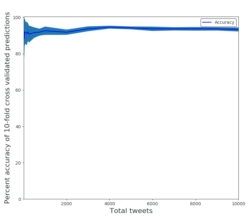
Cross validation is also provided for free, 10-fold cross validation as I’ve used it will split the input feature and label data into 10 groups, and use each of the 10 to build a model to predict on the other 9. You can then get better statistics and not have to worry about localized groupings in the data scewing your results.
With cross validation it’s revealed that even with very low (less than 100) sets of data, Naive Bayes performs extremely well. The results from scikit-learn’s process:
| Tweets Used (from each set) | Accuracy (%) | Deviation (+/-) (%) |
|---|---|---|
| 20 | 93 | 0.23 |
| 30 | 88 | 0.21 |
| 50 | 92 | 0.15 |
| 100 | 92 | 0.12 |
| 200 | 92 | 0.10 |
| 500 | 92 | 0.06 |
| 750 | 92 | 0.04 |
| 1000 | 93 | 0.05 |
| 2000 | 92 | 0.03 |
| 5000 | 94 | 0.02 |
| 10000 | 93 | 0.02 |

References
-
Notes from a Columbia University course focused on Naive Bayes and Maximum Likelihood Estimation.
-
A Chapter from a textbook written by Tom Mitchell at Carnegie Mellon focused on Naive Bayes which also describes discrete valued variables and multiple classes.
-
Andrew Ng’s 5th lecture, on GDA, Naive Bayes, and Laplace Smoothing.
-
Also his 6th lecture, where he discusses multinomial Naive Bayes.
-
And the accompanying notes for the course.
-
Data from a paper out of Texas A&M used for a baseline.
-
One of many Russian twitter troll datasets released by FiveThirtyEight.
-
Code for the demonstration on my Github