Generative Learning and Bayes' theorem

Motivation

I’m getting around to a project implementing a Naive Bayes classifier and there’s some preliminary work that’s going to be helpful in transitioning from logistic and softmax regression algorithms. Hopefully that post can get straight to the code as a result.

Generative vs Discriminate

Discriminant learning algorithms (like logistic regression) try to map from input features to class lables; $P(Y, X=x)$ can be read: the probability of some data point being of a class $y$, given the features $X$ of that point. Conversely, generative learning algorithms try to map classes to the distributions of their features; $P(X, Y=y)$.

To me, the generative side of this symmetry is a little less intuitive. Think of the geographic population distribution of the people who speak French. Already, the word distribution gives it away. “French speaking” is the class label and the geography, be it coordinates or country, is the feature set. You can imagine a good model for French speakers would have a high probability of finding that they have the feature of being from France, and then the DRC, and then Germany, and so on.

It sounds wierd, why would we do such a thing? We want to do it because, having generated such a model, we can use Bayes’ Theorem to retrieve what we typically want to predict, the probability that a person is a French speaker given that they are from a certain country (and of course, other features, if we want a good amount of predictive power).

And its not hard to calculate!

In words:

Thinking of some extreme cases helps feeling our way around this relationship. Imagine a world where 99% of French speakers live in Australia; the numerator on the right becomes very small, and as a result, the feature of being from France wouldn’t be a very strong predictor of speaking French. In another world where 99% of people live in France, the odds of French people speaking French almost becomes simply the odds that a person speaks French in general.

For Example, Gaussian Discriminate Analysis

We do have to come up with some model for the distribution of features. Of course there are infinitely many choices to make here but at least one common choice is to model some dataset as Gaussian, everyone’s favourite distribution. The general form of $k$ dimensional gaussians looks like the following:

If you aren’t familiar with the concept of covariance, Ng has some really nice pictures in his notes that I won’t bother reproducing. Simply put, the matrix describes the shape of the distribution, while the means describe the position.

We can very very easily come up with best fit gaussians for a given datasets and get right to predictions. I’m not even going to prove it, but know that you can in the same way that you usually do, by maximizing the log likelihood of the distributions parameterized by $\mu$ and $\Sigma$. The best fit mean values for a distribution are going to be the mean values of the data points you have available to you, in each direction. The best fit covariance matrix will have terms that simply match the measured covariances between variables in the data points you have available to you.

Code

There’s really not much to see here. The NumPy and SciPy packages contain most of what we want to do in a couple of lines, the rest is just the application of Bayes rule and any matplotlib code I threw together to generate pictures.

	def _predict(self, point, actualClass):
		''' 
		Make the prediction of the class of the point given the point evaluated at the PDF's A and B
		using Bayes rule predictions: P(Y|x) = (P(X|y)*P(y)/(P(x))). Intended for use with only the known data, 
		the points that were used to calculate distA and distB, to predict the values of the remaining points.
		Return 1 if the actualClass(a number, 0:A, 1:B) is equal to the predicted class.
		Return 0 otherwise

		@param point: 		The point, a list-like with 2 members for x and y values
		@param actualClass:	Either 0 or 1, as described above
		'''
		pA = (self.testNumA / (self.testNumA + self.testNumB))
		pB = (self.testNumB / (self.testNumA + self.testNumB))
		pXgivenA = self.gaussDistA.pdf(point) 
		pXgivenB = self.gaussDistB.pdf(point)

		# This term IS unecessary, the argmax evaluation does not 
		# change as it is common between pAgivenX and pBgivenX
		pX = pXgivenA * pA + pXgivenB * pB

		pAgivenX = pXgivenA * pA / pX
		pBgivenX = pXgivenB * pB / pX

		if (pAgivenX > pBgivenX):
			if actualClass == 0:
				return 1
			else:
				return 0
		else:
			if actualClass == 1:
				return 1
			else:
				return 0

Trying it out

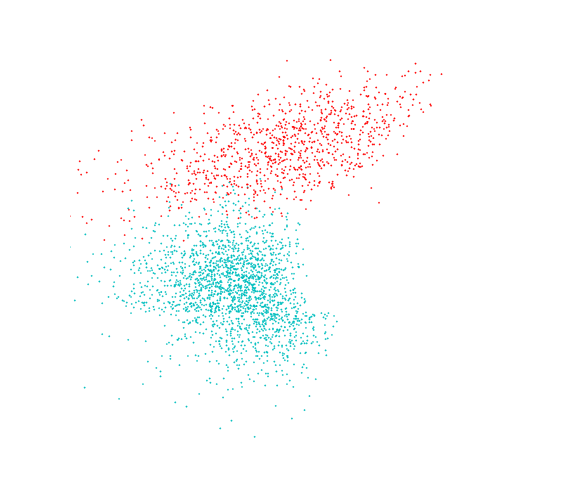
I test out GDA I generated some points again (I promise i’ll be using some real data soon…). Theses aren’t exactly gaussian but they are close. Class A contains contains 2000 and class B contains 1000 points, distributed along two features; this 2:1 ratio shows up in the Bayes calculation. They also mix a little near the boundary so no 100% prediction model will be coming out of this.

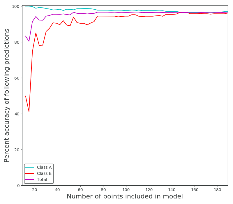
Then it became a choice of how many points from the distribution(s) to sample when forming the original model. I stepped through a range until the results peaked at about 97% correct predictions for both distributions. Interestingly one of the distributions began with 100% accuracy in its predictions, I take this to mean that the distributions formed with low amounts of points (6 from class A, 3 from class B) were so skewed that one of them just dominated the feature space. Of course it over-predicted, and as the second distribution approaches a better fit they even out somewhat.

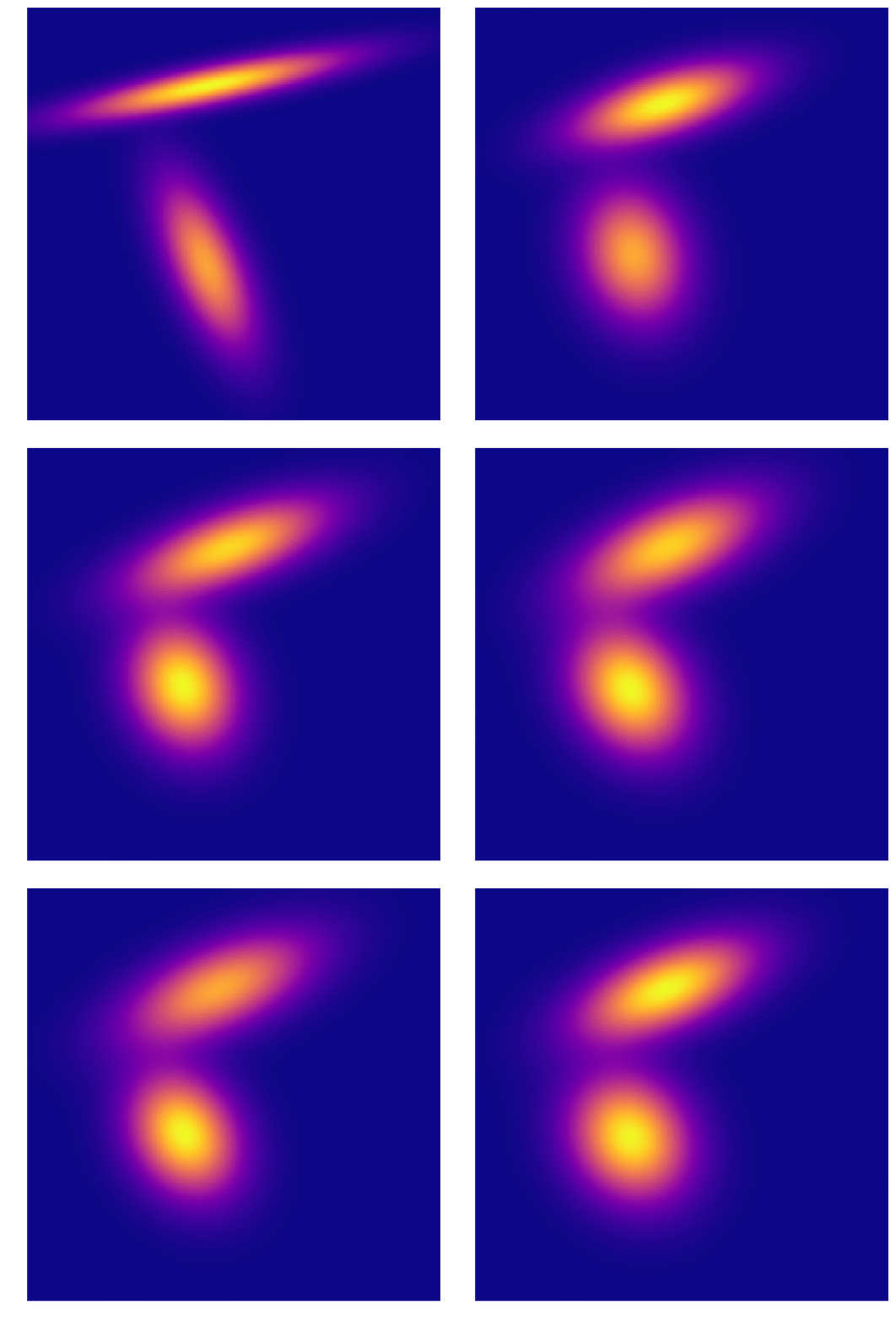
As we all intuitively know, you need large sample sizes to gain predictive power, even for this very simple distribution. And because I can’t help myself, an animation of the distributions associated with the predictions above. In the first frame you can make out the very “sharp” gaussian for class B that causes it to start off in such a poorly predictive state.

References

• Andrew Ng’s lecture on generative learning algorithms, and his notes.

• Code for the demonstration on my Github