Introduction and Motivation
I wanted to revisit a quick topic which was presented to me during my undergrad because it turns out so called Markov Chains are in fact a very useful tool in certain branches of machine learning as well. Additionally, while the basic implementation and proof of concept is entirely possible without any accelerating hardware or algorithm, I still wanted to introduce CUDA to more problems; in this case by upping the dimensionality of the problem. I’ve also gotten CUDA and openGL to play nicely together so I can do away with the pesky third party post-simulation animations, as well as the limiting data transfers from my graphics devices to the host CPU.
The Markov Business
This project is an application of the Metropolis Hastings Algorithm which is of a class of Markov Chain Monte Carlo (MCMC) methods used for deriving probability distrubutions like those found in quantum mechanics. I’ve generally discussed the Markov Chain Monte Carlo in my notes here. The algorithm can be used to discover distributions, given that you know desired properties of the distribution.
Physics
So what distribution are we solving for, and what properties can we take advantage of? This will require some introductory QM work. Everything here can be found in an undergraduate level QM textbook, I’m partial to Griffiths. I’ll cover stationary solutions of the Schrödinger equation (in nice cases) and the Variational Principle which can be used to approximate solutions in some of the less than nice cases. It turns out MCMC will work to discover ground state distrubutions for potentials that we can’t solve analytically. Which turns out to be most real potentials.
We’ll start with the Schrödinger equation itself, a second order differential equation:
It describes the evolution of a wave-function, $ \Psi $ in time, in response to its initial conditions and the potential $V$. $ \Psi $ itself is a quantum mechanical description of a particle; no longer discrete but distributed in space with some probability of observing it in a given region. The wave-function itself is not physical, it’s more of a mathematical artefact; what really matters are observable quantities like the expected position, which can be calculated
There are any number of solutions to the equation, but it turns out that there exists a class of solutions which are time independant, and that these solutions are very important. Through separation of variables and some substitution the Schrödinger equation can be split into two ordinary differential equations of time and of position:
You can solve the time dependant equation easily though integration and write out our new $ \psi $:
Functions of this form have a stationary probability density. (That term under the integral before). The complex exponential terms cancel as per Euler’s formula.
So the wave functions which satisfy the product form of the Schrödinger equation correspond to stationary states. Not only the expected position, but all observable quantities are constant for these states; the expected energy is constant, and of course momentum which is zero for a stationary state. Most importantly these stationary solutions are eigenfunctions - or eigenvectors if you like - of the observables of the state as represented by hermitian operators. This means that the general time-independant Schrödinger equation, can be written as a linear combination of the stationary states written above. So, Thats a lot of linear algebra in a few sentences, and unfortunately I won’t be proving or going into more detail here. I’d recommend the back of Griffiths for a very brifef, physics-relevant view; or any math textbook on the subject if you are curious.
Ok cool, if we’ve found the eigenstates of the system, we’ve in fact solved for states which are time dependant as well, as they can be written as a weighted sum of stationary states, which is of course normalized. However, it turns out that outside of certain cases we cannot solve for these states analytically. Instead we often have to rely on numerical methods.
Speaking of numerical methods; we should find a proof of the Variational Principle some chapters into our favorite QM textbook. For cases not included in the link above, we can resort to using the Variational Principle to calculate at least an upper bound on the ground state energy and corresponding eigenfunction for a particular potential. It goes as follows, for any normalized wave-function $\psi$, which we can choose at random
In words, this must be true because we know we can decompose our chosen $\psi$ into an equivalent sum of orthogonal eigenstates. Any eigenstate which takes part in this series and is also not the ground state will be contributing more energy than it would have if it had been the ground state to begin with, by definition of the ground state being the lowest energy eigenstate.
In less words, while any $E_n \geq E_0$:
Thats it for the physics. The property we were looking for to use in the MCMC algorithm is exactly the property described by the Variational Principle. A physicist can make educated guesses as to the trial function to use, and even provide that function with tuning parameters to minimize the rezulting energy for the form of the function. However, introducing MCMC as i’ve described here will allow us to explore the entire space of possible distributions. So now we can get to the code and results.
Code Samples
	 /* measure the action change and roll for a result
	 * if necessary. This metd just compacts the repeated uses
	 * within Step() */

__device__ float2 MCTest(float2* rawRingPoints,
						 float2 newPoint,
						 int mode,
						 float tau,
						 float dt,
						 int numPoints,
						 unsigned int thdIdx)
{
	curandState state;
	curand_init((unsigned long long)clock(), thdIdx, 0, &state);
	float S_old = Action(rawRingPoints, rawRingPoints[thdIdx], mode, dt, numPoints, thdIdx);
	float S_new = Action(rawRingPoints, newPoint, mode, dt, numPoints, thdIdx);
		// If action is decreased by the path always accept
	if(S_new < S_old)
	{
		return newPoint;
	}
		// If action is increased accept w/ probability
	else
	{
		float roll = curand_uniform(&state);
		float prob = expf(-S_new/(1.0/tau)) / expf(-S_old/(1.0/tau));
		if(roll < prob){
			return newPoint;
		}
	}
	return rawRingPoints[thdIdx]; // simply return the existing point
}

		/* Steps alternating even/odd "red/black" points in the path
		 * with the chance of acceptance being related to the change
		 * in the action which the move brings to the path */
		// Note: Kernel Functions can't be defined within the class

__global__ void Step(float2* rawRingPoints,
					 float epsilon,
					 int mode,
					 float tau,
					 float dt,
					 int numPoints,
					 unsigned int redBlack)
{
	int idx = blockIdx.x * blockDim.x + threadIdx.x;
	if (idx >= numPoints)
		printf("ERROR: Out of rawRingPoints[] bounds, calling: %d, max: %d\n", idx, numPoints);

	// alternate steps, red/black:
	if((idx + redBlack) % 2 == 0)
	{
		return;
	}

	float2 newPoint = rawRingPoints[idx];

	curandState state;
	curand_init((unsigned long long)clock(), idx, 0, &state);

	float randX = (0.5 - curand_uniform(&state)) * 2.0 * epsilon;
	float randY = (0.5 - curand_uniform(&state)) * 2.0 * epsilon;
	newPoint.x = rawRingPoints[idx].x + randX;
	newPoint.y = rawRingPoints[idx].y + randY;

	// Run accept/deny on the move
	rawRingPoints[idx] = MCTest(rawRingPoints, newPoint, mode, tau, dt, numPoints, idx);
	__syncthreads();
}
I forgot to mention that rather than using the energy of a particle as the quantity of interest for MCMC, I have used the action of its path instead. It is equivalently minimized given a certain Wick Rotation has been applied to the state $\psi$. Given that you view many paths, this results in the same distribution and lowest eigenenergy.
Results
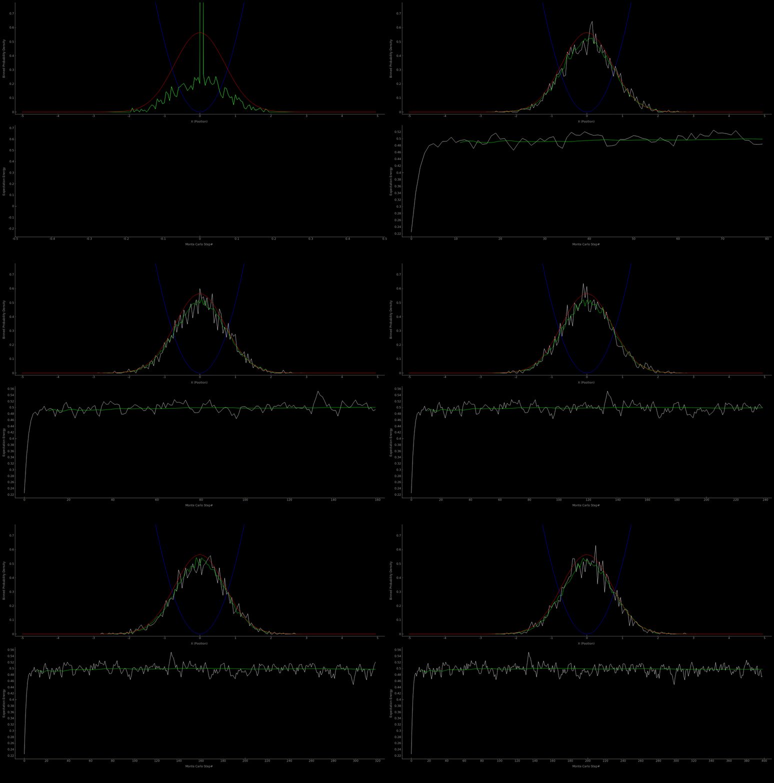
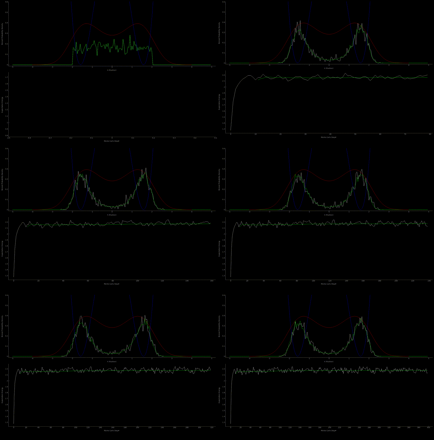
The following two outputs come from a python script implementation of the algorithm; it’s not so computationally expensive to get good results in one dimension for fairly simple potentials:


At this point I wanted to implement the algorithm in higher dimensions and with a nicer visualization. Honestly I spent too much time here, but I got to learn more CUDA - openGL interoperability which is always great for visualization when running GPU accelerated algorithms:

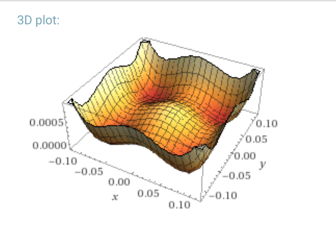
I also tried a potential with four nodes, as an extension to the double well potential. I suppose this might make for a crude model of a very small lattice potential, but I wouldn’t claim it’s representational of any real physical system (as if that has ever stopped anybody). It looks like this, with the following form and a plot from wolfram alpha:


References
-
An introduction to the Markov Chain detail balance
-
Or a wiki page on the topic if you want to scratch that itch with less math.
-
And finally, an introductory Khan video provides a great example to introduce the topic.
-
Introduction to Quantum Mechanics, 2nd ed. David Griffiths