N-Body Simulations for Galaxies - CUDA

Introduction and Motivation

Following up after the simplified model in the previous post, I can now get into more high powered applications. The only “new physics” to be discussed at this point is the new model for the galaxies, which will be random populations of density functions which have been granted to us by Kiujiken & Dubinski. We also introduce dark matter to our galaxies, which turns out to be a necessity for stability.

The simulation on the other hand requires a new approach; using the parallelism of CUDA to cut down on the extremely expensive simulation times. With the number of masses I intended to use, the straightforward CPU based approach (without any fancy speed ups ) simulations of a reasonable time-scale would have taken lifetimes! Particularly on my poor little laptop. I’ll be discussing the technology behind GPU computing and the CUDA based algorithm which allows for these simulations to be ran in hours, or minutes really, if you don’t want to bother making smooth videos like I did.

There is quite a bit of motivation for this work for me personally, GPU computing opens doors to a new scope of computational science, in areas like fluid dynamics, quantum electrodynamics (QED), and molecular dynamics.

The Physics

I’ll break this portion into descriptions of Kiujiken & Dubinski’s models for the bulge, halo, and disk which I have generated to use as initial conditions. The bulge and halo are simpler, nearly spherically symmetric models which are approximately stable on their own, the rings are more complex due to their asymmetry. The functions I post below are distribution functions in energy which have density functions (the probability to be found in a region of phase space which one would expect to use to populate at random) associated with them through integration over 2 or 3 variables, depending on the model. The paper solves for these functions as well.

The Bulge

The bulge utilizes King’s model, which can be thought of as a truncated Isothermal Sphere. Model’s such as these achieve stability by requiring inward gravitational forces to match outward “pressure” when forming a distribution. One must make corrections to an infinity which arises at the origin, as well as the truncation which must be made in a simulation, without which the sphere would go to infinity and contain theoretically infinite mass. Here’s what that ends up looking like in the paper:

These are not very pretty! What matters here are the desired ρb value specifying the central bulge density, and the relationships between ψc and σb and σ0, which determine how sharply the distribution cuts off. The author’s chose values which gave a more centrally dense bulge than the halo distribution, likely to match observation.

The Disk

The model for the disk expects there to be central mass, from the bulge and halo, in order to be stable. As such, masses closest to the center are given more energy such that they don’t collapse inward. Simulating the thing alone the results in an expansion of these masses, but I’ve done it anyway for the sake of completion. The distribution function below has become a function of 3 energy variables, w.r.t. planar motions, angular momentum, and the additional z energy component which the paper models simply as an oscillation across the plane of the disk:

the density and frequency parameters with a tilde are chosen to match observations, in particular light densities and rotation speeds of real disk galaxies, and likely for stability as well when the disk model is mixed with the other two. Energies and frequencies as a function of Rc are dependent on the energy of a circular orbit with the desired Lz parameter.

The Halo

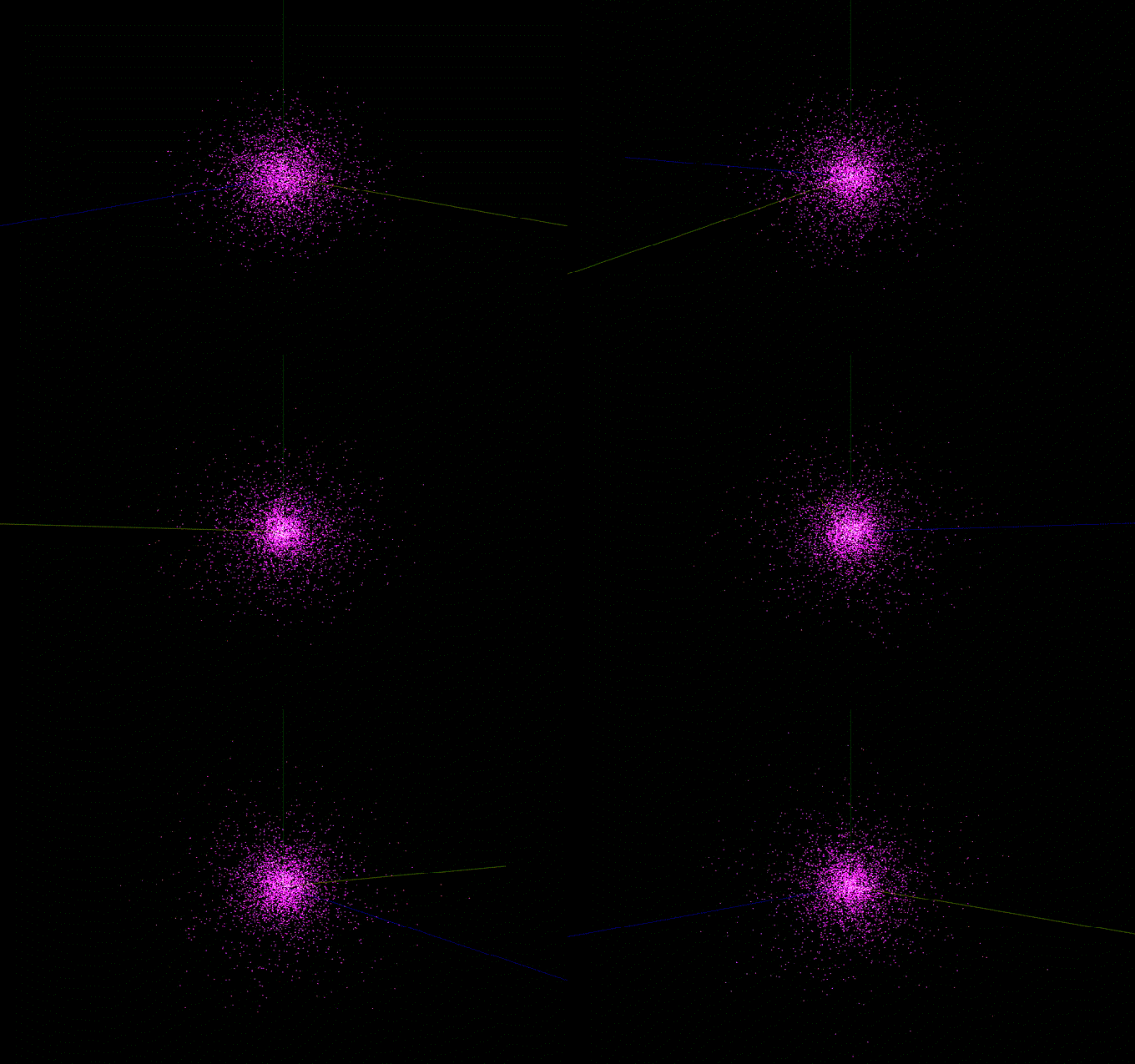
If you can make out the now tiny axes (which have remained the same size) through the artifacts in the gif you can see the halo is massive in comparison to the visible galaxy. It’s also literally massive, ~94% of the entire system using this combined model. The distribution function is not too different from that of the bulge, it decays more slowly and most importantly, it is not spherical. It’s known as an Evan’s model and has slightly flattened poles, converging slightly inward towards the disk

As described, the parameters A, B, and C, correspond to the density scale, the “core” radius, and the flattening parameter which is characteristic of Evan’s model.

All Together

The Code

The CUDA device code i’ve used is shown below. As demonstrated by NVDIA, the acceleration kernel is split into chunks (“tiles”) which can access a smaller pool of shared memory while they run. The other kernels perform the leapfrog steps of the algorithm after acceleration has been calculated for each body.

		/* Single body-body interaction, sums the acceleration 
		 * quantity across all interactions */
__device__ float3
bodyBodyInteraction(float4 bi, float4 bj, float3 ai, float softSquared) 
{
	float3 r;
	r.x = bj.x - bi.x;
	r.y = bj.y - bi.y;
	r.z = bj.z - bi.z;
	float distSqr = r.x * r.x + r.y * r.y + r.z * r.z;
	float invDist = rsqrt(distSqr + softSquared);
	float invDistCube = invDist * invDist * invDist;
	float s = bj.w * invDistCube;
	if(r.x != 0.0){
		ai.x += r.x * s;
		ai.y += r.y * s;
		ai.z += r.z * s;
	}
	return ai;
}

		/* Apply body-body interactions in sets of "tiles" as per
		 * NVIDIA's n-body example, loading from shared memory in 
		 * this way speeds the algorithm further */ 
__device__ float3
tile_accel(float4 threadPos, float4 *PosMirror, float3 accel, float softSquared,
		   int numTiles) 
{

	extern __shared__ float4 sharedPos[];

	for (int tile = 0; tile < numTiles; tile++){
		sharedPos[threadIdx.x] = PosMirror[tile * blockDim.x + threadIdx.x];
		__syncthreads();

#pragma unroll 128

		for ( int i = 0; i < blockDim.x; i++ ) {
			accel = bodyBodyInteraction(threadPos, sharedPos[i], accel, softSquared);
		}
		__syncthreads();
	}
	return accel;
}

		/* Acquire all acceleration vectors for the points */ 
__global__ void
accel_step( float4 *__restrict__ devPos,
			float3 *__restrict__ accels,
			unsigned int numBodies,
			float softSquared,
			float dt, int numTiles ) 
{
	int index = blockIdx.x * blockDim.x + threadIdx.x;
	if (index > numBodies) {return;};
	accels[index] = tile_accel(devPos[index], devPos, accels[index], softSquared, numTiles);
	__syncthreads();
}

		/* Step all point-velocities by 0.5 * a * dt
		 * as per a leapfrog algorithm; is called twice,
		 * once before and once after the position step */
__global__ void
vel_step( float4 *__restrict__ deviceVel,
		  float3 *__restrict__ accels,
		  unsigned int numBodies,
		  float dt)
{
	int index = blockIdx.x * blockDim.x + threadIdx.x;
	if (index > numBodies) {return;};
	deviceVel[index].x += accels[index].x * 0.5 * dt;
	deviceVel[index].y += accels[index].y * 0.5 * dt;
	deviceVel[index].z += accels[index].z * 0.5 * dt;
}

		/* Step positions from velocities */
__global__ void
r_step( float4 *__restrict__ devPos,
		float4 *__restrict__ deviceVel,
		unsigned int numBodies,
		float dt)
{
	int index = blockIdx.x * blockDim.x + threadIdx.x;
	if (index > numBodies) {return;};
	devPos[index].x += deviceVel[index].x * dt;
	devPos[index].y += deviceVel[index].y * dt;
	devPos[index].z += deviceVel[index].z * dt;
}

		/* zero the acceleration array between leapfrog 
		 * steps, I wasn't sure if a cuda mem-set existed 
		 * and/or would be faster */
__global__ void
zero_accels( float3 *__restrict__ accels ) 
{
	int index = blockIdx.x * blockDim.x + threadIdx.x;
	accels[index].x = 0.0f;
	accels[index].y = 0.0f;
	accels[index].z = 0.0f;
}

These are all called with the same thread dimensions using CUDA’s kernel launch syntax:

const int threadsPerBlock = 512;		// blockSize from NVDA_nbody
const int numTiles = (numPoints + threadsPerBlock -1) / threadsPerBlock;
const int sharedMemSize = threadsPerBlock * 2 * sizeof(float4);

. . .
. . .

	// the leapfrog algorithm through CUDA kernel calls:

accel_step <<< numTiles, threadsPerBlock, sharedMemSize >>>
		   (dev_points, dev_accels, numPoints, softSquared, dt, numTiles);

vel_step <<< numTiles, threadsPerBlock, sharedMemSize >>>
		 (dev_velocities, dev_accels, numPoints, dt);

r_step <<< numTiles, threadsPerBlock, sharedMemSize >>>
	   (dev_points, dev_velocities, numPoints, dt);

vel_step <<< numTiles, threadsPerBlock, sharedMemSize >>>
		 (dev_velocities, dev_accels, numPoints, dt);

zero_accels <<< numTiles, threadsPerBlock, sharedMemSize >>>
		   (dev_accels);

References

• The Disk-Bulge-Halo model for galaxies, stability, etc: Kiujiken & Dubinski

• Their GalactICS package which I have used to populate galaxies is publicly available

• My GitHub repo for this project