Motivation
Lessons on Support Vector Machines - at least the ones I’ve watched - jump straight into a lagrangian representation for a constrained miminization problem without much justification. I thought it would be valuable to prove to myself why this approach works, before going on to use it in SVM classification later.
Minimizing one function with one constraint
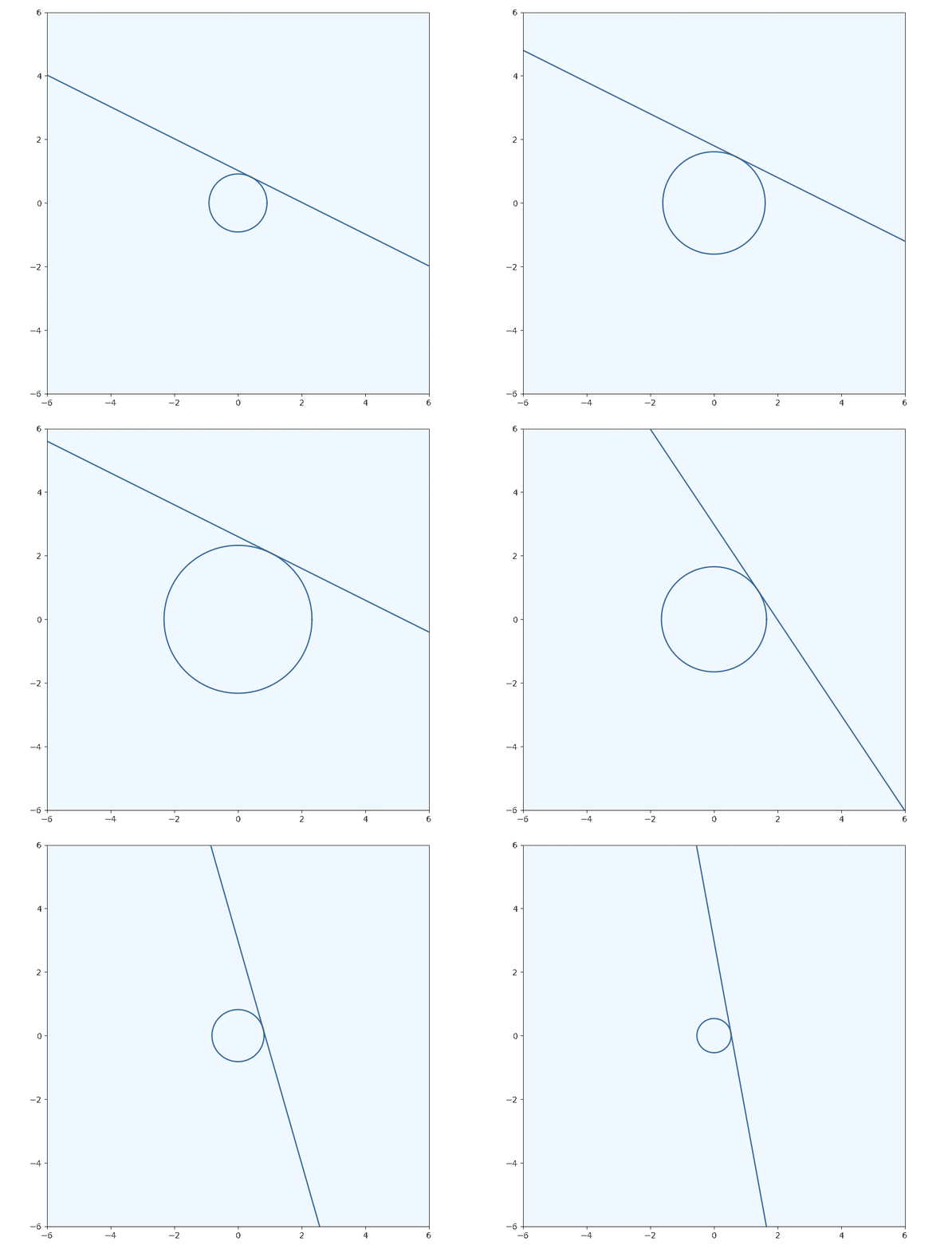
I’ll use a 2d parabola as the function I’m trying to minimize, with the inequality constraint of . I’ll call the line of the inequality and for now I’ll be assuming that the minima will actually lie on this constrianing line and ignore the fact that it’s an inequality.
To minimize, we want to decrease as long as we can while the still satisfying the inequality (intersecting with the constraint at least once). The minima will occur when we have just one single point left which satisfies our constraint

A fact we can use to solve for this point of interest is that tangent curves will have gradients which are proportional to eachother.
With the addition of the constraint equation itself we then have 3 variables and 3 equations which we can solve. In this case we could just substitute our way to the solution, but with higher dimensional functions with increasing numbers of variables it helps to make use of gaussian elimination strategies. And of course, any software employing these methods can make use of LAPACK or Numpy’s linalg module (also lapack) to solve the system:

The “Lagrangian” in the name of this method just refers to the form of the system of equations when written out to one side, and the “multipliers” are just what people call the extra variables we introduce, $\lambda$.
Any constant term in the constraint is moved from the right to the left under the multiplier; such that $ \lambda (g(x, y) - b) = 0 $. This is one of the KKT conditions known as complementary slackness. “Slackness” is used because when the constriant is found to be more than satisfied the behavior of the system allows for it; essentially allowing for some “cost” to accumulate as a result.
What about when constraints don't matter?
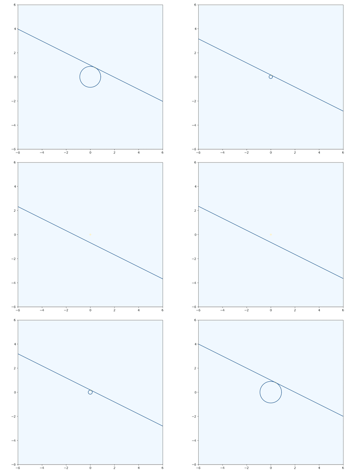
Now I’ll let $g(x,y)$ be the inequality $y + \frac{1}{4}x - 1 \geq 0$ and not assume that the solution lies on the constraint boundary. With a constraint on the system that’s not binding - the minima of the function lies within the constrained region but not on the boundary - the system of equations to solve becomes the usual $\nabla f(x, y) = \vec{0}$. This is entirely contained by the form of the Lagrangian. Taking the derivative of the Lagrangian and setting it to zero is conveniantly equivalent to stating the system of equations that we found above:
But if $lambda$ is zero, as is the case for a non-binding constraint, you are left with the usual minimization equation:

We know to set $\lambda$ for the constraint to zero when the inequality constraint is more than satisfied; $g(x,y) > 0$. Think about it from a calculus perspective, if the value of the constraint is currently positive by any amount, then moving anywhere in the feature space by any infinitesimally small amount you will still have a $g(x,y)$ value that is greater than zero, and so we must be in the region enclosed by the inequality and not on the border - not bounded. That assumption wouldn’t hold for non-continuous constraints, so don’t use those unless you want to come up with clever workarounds. An equivalent reason for setting $\lambda$ to zero arises when discussing the lagrangian in terms of the primal and dual problem, which I’ll get to later.
What about multiple constraints?
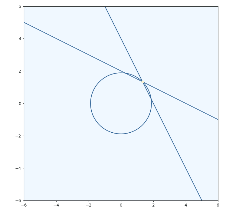
Lets say we had two constriants on the same function as before; $ \frac{1}{2}x + y + 2 \geq 0 $ and $ 2x + y + 4 \geq 0 $. We end up just adding to the lagrangian:
We then go and solve the system of derivatives just as we did before, we just have a larger matrix equation in front of us.

We’re not done at this point. We can already imaging the awkward situation which results when we go ahead and add more constraints, with some binding and some non-binding, which may not have a conveniant shared solution of this form. Later, the dual optimization problem, the addition of a tolerance factor, and the application of sequantial minimalization methods will finally bring us to the point of solving an arbitrary system.