Softmax Regression

Motivation

Logistic regression only worked with two classes, surely we should be able to distinguish between more. This post will contain a description of the softmax regression algorithm with a proof that gets us from the hypothesis function to the weight update rule which comprises the algorithm. I’ll also discuss the code for this project which utilizes CUDA to speed up the main update algorithm, as well as visualization functions. This particular implementation is general in the number of classes for our data, but specifically expects two input features, so that we can plot them easily. To grow the input feature set would be to grow a vector here or there.

Exponential Family to Retrieve the Softmax Hypothesis Function

As with all these regressions, we are attempting to apply gradient descent to the parameters of a hypothesis function such that likelihood is maximized. Before, the sigmoid function of logistic regression was ideal in that it had an output on $[0, 1]$ and could distinguish between two regions. It turns out that the sigmoid can be retrieved generally from inverting a certain natural parameter of a probability distribution which lives in the exponential family. The exponential family contains probability distributions parameterized by $\eta$ (the natural parameter) in the following form:

$$ p(y|\eta) = h(y)e^{\eta^TT(y)-A(\eta)} $$

Where the inclusion of the inner product lets us know that $\eta$ can generally be a vector; this turns out to be the case now that we are attempting to generate a model for multiple classes. There’s quite a few terms here: $h(y)$, a normalization term, $T(y)$ the sufficient statistic, $A(\eta)$ the cumulant function, and our natural parameter $\eta$. I won’t go into detail about the sufficient statistic or cumulant function here, they have very useful properties which are detailed in the Berkeley link.

Often you want to represent the parameter vector $\eta$ as a linear combination of the form:

$$ \vec{\eta} = \phi(\theta) \\ \text{and so:} \\ p(y|\phi(\theta)) = h(y)e^{\phi(\theta)^TT(y)-A(\phi(\theta))} $$

Though of course there are cases where $\eta$ cannot be represented in this way, these cases are considered non-linear or of the curved exponential family. I’m also not dealing with those here.

If however we can represent our probability in this way, our hypothesis function falls out of the exponential family form by inverting the parameter vector; now $\phi(\theta)$. All we have to do first is convert our probability function into the form of the exponential family. There’s a really neat trick, simply taking the exponent of the log of the probability will get you most if not all the way there. For example, when classifying between two cases $y=0$ and $y=1$ in the previous post we used the Bernoulli distribution. Using the trick:

$$ \begin{align}p(y | \phi) & = \phi^y(1 - \phi)^{1-y} \\ &= e^{y log(\phi) + log(1-\phi)} \\ \end{align} $$

Which gives us the forms of the functions:

$$ \eta = log(\frac{\phi}{(1-\phi)}) \\ T(y) = y \\ A(\eta) = -log(1 - \phi) = log(1 + e^{\eta}) $$

And inverting the equation for $\eta$:

$$ \phi = \frac{1}{1+e^{-\eta}} $$

Which was exactly the logistic hypothesis function from before.

Now for multiple classes we have a new multinomial probability distrubution to try out. For $M$ trials on data comprised of $K$ classes

$$ p(y | \phi) = \frac{M!}{\prod_{k=1}^K{y_k!}}\prod_{k=1}^K{\phi_k^{y_k}} $$

First drop the scaling factor out front and focus only on the product of the natural parameters $\phi$. We can use the same trick on this form of the equation. We also break out the $K^{th}$ component of $\phi$ from the rest of the sum to achieve a minimal representation for the distribution. This makes sense; as Ng describes in his notes, once we have up to $K-1$ terms, the $K^{th}$ term can be represented by one minus the sum of the rest. Using that replacement:

$$ \begin{align} p(y | \phi) &= \exp \Big\{ \sum_{k=1}^{K} y_k \log{\phi_k} \Big\}\\ & = \exp\Big\{\sum_{k=1}^{K-1}y_k\log\Big\{\phi_k\Big\} + (1-\sum_{k=1}^{K-1}y_k)\log\Big\{1-\sum_{k=1}^{K-1}\phi_k\Big\}\Big\} \\ & = \exp\Big\{\sum_{k=1}^{K-1}y_k\log\Big\{\phi_k\Big\} - \sum_{k=1}^{K-1}y_k\log\Big\{1-\sum_{k=1}^{K-1}\phi_k\Big\} + \log\Big\{1-\sum_{k=1}^{K-1}\phi_k\Big\}\Big\} \\ & = \exp\Big\{\sum_{k=1}^{K-1}\log\Big\{\frac{\phi_k}{1-\sum_{k=1}^{K-1}\phi_k}\Big\}y_k + \log\Big\{1-\sum_{k=1}^{K-1}\phi_k\Big\}\Big\} \\ \end{align} $$

Where in the last line we’ve retrieved the form of the exponential family and we get each of our $k$ hypothesis functions by inverting the natural parameter and solving for $\phi_k$, making the same assumption that $\eta$ is a linear combination of weighted terms $\vec{\theta_k}^{T}\vec{x}$ for weights associated with each class:

$$ \eta_k = \log\Big\{\frac{\phi_k}{1-\sum_{k=1}^{K-1}\phi_k}\Big\} \\ \phi_k = \frac{e^{\eta_k}}{\sum_{j=1}^{K}e^{\eta_j}} \\ or \\ \phi_k = \frac{e^{\vec{\theta_k}^{T}\vec{x}}}{\sum_{j=1}^{K}e^{\vec{\theta_k}^{T}\vec{x}}} \\ $$

There’s probably a better way to get vector transposes to display through LaTeX . . . i’ll drop the arrow from now on but keep it in mind

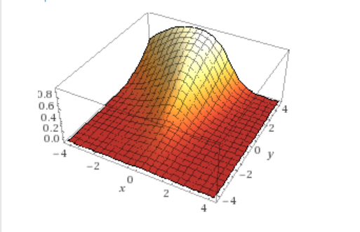
Pictures always help so here’s what that function looks in two dimensions for $\theta$ weights $[1, 1], [3, 0.5]$ plotting for the first class, you can think of it as a region selector for your feature space:

Getting a feel for the form of the hypothesis function

Derivative of Log Likelihood to Retrieve Update Rule

Remembering that the general form of log likelihood maximization goes:

$$ \theta := \theta + \alpha\nabla_{\theta}L(\theta) $$

we’ll need to get the likelihood function and take its derivative. What we recovered above was the hypothesis function for a point of a class $k$ (note the subscript). The function for all classes must represent the joint probability of the classes at hand. When you have joint probabilties, you multiply the individual terms. Go ahead and check if that doesn’t make sense. Because of this, the likelihood function this time around must be a product. Remeber that before, for logistic regression between two classes, it was a sum. Here’s what that looks like:

$$ \begin{align} L(\theta) &= \prod_{i=1}^{m}p(y_i | x_i; \theta) \\ &= \prod_{i=1}^{m}\phi_1^{I\{y_i=1\}}...\phi_K^{I\{y_i=K\}} \end{align} $$

Where

$$ \phi_k = \frac{e^{\theta_k^{T}x}}{\sum_{j=1}^{K}e^{\theta_k^{T}x}} $$

And $I{y_i = n}$ is an indicator function, just the boolean test: $class\space of\space point == this\space class$. This is just a nice way of representing the joint probability. At this point I definitely lost track of subscripts and products and I didn’t have a very good feel for what the function was doing. If you feel this way, here is it written very explicitely for a dataset of 5 points, of three classes, defined by two features. Points $[1,2,3,4,5]$ are of classes $[1,1,2,3,3]$ in this example, and take on features $[x, y]$

$$ L(\theta_k) = \phi_1(\vec{X_1}) + \phi_1(\vec{X_2}) + \phi_2(\vec{X_3}) + \phi_3(\vec{X_4}) + \phi_3(\vec{X_5}) \\ L(\theta_k) = \frac{e^{\theta_k^TX_1}}{1+\sum_{j=1}^{K-1}e^{\theta_j^TX_1}} + \ldots + \frac{e^{\theta_k^TX_5}}{1+\sum_{j=1}^{K-1}e^{\theta_j^TX_5}} $$

I’ll return to this pretend set of data to write out the derivative term explicitely. Speaking of the derivative (of the log):

$$ \begin{align} L(\theta) & = \prod_{i=1}^{m}\phi_1^{I\{y_i=1\}}...\phi_K^{I\{y_i=K\}} \\ log(L(\theta)) & = \sum_{i=1}^m\theta_k^TX_i - log(1+\sum_{j=1}^{k-1}e^{\theta_j^TX_i}) \\ \frac{\partial{log(L)}}{\partial{\theta_{k}}} & = \sum_{i=1}^mI\{X_k == k\}X_i - \frac{X_ie^{\theta_{k}^TX_i}}{1+\sum_{j=1}^{K-1}e^{\theta_j^TX_i}} \\ \\ \text{Or, individually for each feature j:} \\ \frac{\partial{log(L)}}{\partial{\theta_{jk}}} & = \sum_{i=1}^mI\{X_k == k\}X_{ij} - \frac{X_{ij}e^{\theta_{k}^TX_i}}{1+\sum_{j=1}^{K-1}e^{\theta_{jk}X_{ij}}} \\ \end{align} $$

Note that the Indicator function fell out here when taking the derivative of the lone inner product on the left with respect to $\theta_k$. Then if we just factor out the common $X_{ij}$ term we have our update rule:

$$ \boxed{\theta_{jk} := \theta_{jk} + \alpha\sum_{i=1}^mx_{ij}\Big(I\{k==X_k\} - \frac{e^{\theta_{jk}^Tx_{ij}}}{1+\sum_{j=1}^{K-1}e^{\theta_{jk}^Tx_{ij}}}\Big ) } $$

Note that our parameter weights now come in the form of a matrix of dimensions $j\space x\space k$ for each $k$ class and $j$ feature, so a full iteration of gradient descent now must take this derivative term for all points $j\cdot k$ times.

To illustrate what the derivative looks like explicitely, for the same pretend weights from before, when taking the derivative with respect to $j=x$ and $k=1$

$$ \frac{\partial{log(L)}}{\partial{\theta_{1,x}}} = X_{1,x}\Big(1 - \frac{e^{\theta_{1,x}^TX_{1,x}}}{1+e^{\theta_{1,x}^TX_{1,x}}+e^{\theta_{2,x}^TX_{1,x}} + \ldots} \Big) + \ldots + X_{1,x}\Big(0 - \frac{e^{\theta_{1,x}^TX_{3,x}}}{1+e^{\theta_{1,x}^TX_{1,x}}+e^{\theta_{2,x}^TX_{1,x}} + \ldots} \Big) $$

Note the difference between the two terms; as a result of the state of the indicator terms for the various derivative sums, the derivative will approach zero as $\vec{\theta}$ causes the function to encapsulate points of the class, and as it excludes points not of the class. This is nice, we won’t get false positives!

Hopefully that does it for the mathy bits for this post. As usual, all we really needed was the update rule in the box above; but we really wouldn’t have known how to come up with these things in the future then would we?

Code

The CUDA kernel that calculates the derivative terms for every point is really the crux of the algorithm. Much of the rest of the code is really just calculating and scalling the resulting probability field so it can be displayed through openGL interoperability. Here’s that kernel and its launch:

	// DivLogLikelihood_Kernel.cu

	/**
	 * Performs dLogL on classed data with 2 features, 
	 * populating vectors of derivative terms for summation later
	 * in the algorithm. This function should be called once for each 
	 * class of points, asynchronously if you have the device memory for it.
	 * @param points        A device pointer to the float2 data
	 * @param dxTerms       A device pointer to be populated with derivative terms corresponding to the first feature "x"
	 * @param dyTerms       A device pointer to be populated with derivative terms corresponding to the first feature "y"
	 * @param devWeights    A device pointer to the parameter weights (Theta's) at the current iteration, float2 x numClasses
	 * @param numPoints     The total number of points per class, for bounds checking with maximum thread index
	 * @param classNum      The class number for which the derivative is being calculated.
	 * @param numClasses    THe total number of classes in the model
	 **/

	__global__ void divLogLikelihood(const float2* __restrict__ points,
	                                 float*        dxTerms,
	                                 float*        dyTerms,
	                                 float2*       __restrict__ devWeights,
	                                 const int     numPoints,                   // number of points in a class                              (m / numClasses)
	                                 const int     classNum,                    // the index of the class of the weight being operated on   (k)
	                                 const int     numClasses)                  // the total number of classes                              (K)
	{
	    int pointIdx = blockIdx.x * blockDim.x + threadIdx.x;                   // the index of the point                                   (i)
	    if (pointIdx >= numPoints * numClasses) { return; }     // out of array bounds check

	        // determine class of the point. I didn't take up data for this 
	        // the points are just sorted by class in blocks of length #numPoints
	        // Obviously a real data set could be sorted and bookmarked to achieve this.

	    int pointClass = static_cast<int>(pointIdx / numPoints);
	    float indicatorTerm = 0.0;
	    if (pointClass == classNum)
	    {
	        indicatorTerm = 1.0;
	    }

	    float2 point = points[pointIdx];
	    float expxTerm = 0.0;
	    float expyTerm = 0.0;
	    float sumxTerm = 0.0;
	    float sumyTerm = 0.0;

	    expxTerm = expf(devWeights[classNum].x * point.x);
	    for (int classIdx = 0; classIdx < numClasses; ++classIdx)
	    {
	        sumxTerm += expf(devWeights[classIdx].x * point.x);
	    }
	    float testx = point.x * (indicatorTerm - (expxTerm / (1.0 + sumxTerm)));
	    dxTerms[pointIdx] = testx;

	    expyTerm = expf(devWeights[classNum].y * point.y);
	    for (int classIdx = 0; classIdx < numClasses; ++classIdx)
	    {
	        sumyTerm += expf(devWeights[classIdx].y * point.y);
	    }
	    float testy = point.y * (indicatorTerm - (expyTerm / (1.0 + sumyTerm)));
	    dyTerms[pointIdx] = testy;   
	}

The derivative kernel is called in a driving loop alongside visualization code. Here’s the important part of the loop that corresponds to the algorithm. Thrust is great for fast reduction algorithms like sums and filling operations.

		// Take dLogL for each class, filling each derivative vector

	for (int classIdx = 0; classIdx < mSettings->numClasses; ++classIdx)
	{

		divLogLikelihood<<<mRegressionBlocks, mRegressionTPB>>> 
			(mData->devPointsPtr,
			 mData->devDivLogLPtrs[classIdx][0],	// x divs
		     mData->devDivLogLPtrs[classIdx][1],	// y divs
		     mData->devWeightsPtr,
		     mSettings->numPoints,																																	 
  		     classIdx,
  		     mSettings->numClasses);
			
		gpuErrchk(cudaDeviceSynchronize());
	}

	gpuErrchk(cudaDeviceSynchronize());

		// Sum the derivative vectors

	for (int classIdx = 0; classIdx < mSettings->numClasses; ++classIdx)
	{
		for (int featureIdx = 0; featureIdx < mSettings->numFeatures; ++featureIdx)
		{
	        dLogLSums[classIdx][featureIdx] = thrust::reduce(mData->devDivLogLTerms[classIdx][featureIdx].begin(), 
	        									             mData->devDivLogLTerms[classIdx][featureIdx].end());						  				  		 
		}
	}

	gpuErrchk(cudaDeviceSynchronize());

		// reset the derivative vectors for the next iteration

	for (int classIdx = 0; classIdx < mSettings->numClasses; ++classIdx)
	{
		for (int f = 0; f < mSettings->numFeatures; ++f)
		{
			thrust::fill(mData->devDivLogLTerms[classIdx][f].begin(), 
				         mData->devDivLogLTerms[classIdx][f].end(),
				         0.0);
		}
	}	

		// update the weights using the sums and scaling factors

	for (int classIdx = 0; classIdx < mSettings->numClasses; ++classIdx)
	{
		mData->hostWeights[classIdx].x += mData->hostAlphas[classIdx].x * dLogLSums[classIdx][0];
		mData->hostWeights[classIdx].y += mData->hostAlphas[classIdx].y * dLogLSums[classIdx][1];
	}

		// copy the updated weights from the host to the device for the next iteration

	mData->devWeights = mData->hostWeights;
	mData->devWeightsPtr = thrust::raw_pointer_cast(mData->devWeights.data());

The rest of the code is just management of data and kernels to produce the following visualizations.

Results

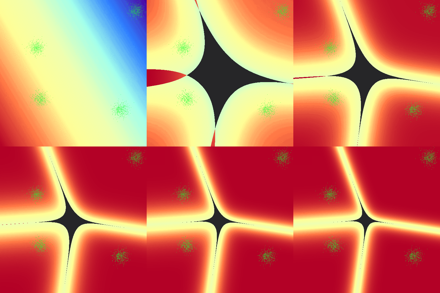
First, a nice pretty run with really low $\alpha$ values to capture the behavior of the regression. Here i’ve cut each of the distributions $\phi_k$ at the point where they dip below 50%, and then normalized each $\phi$ such that I could scale color with probability. I haven’t yet looked for real data to run this on, for visualization purposes it would have to be something trivial with two features. For now I’m just using some generated guassians with 512 points per class (nice cuda numbers).

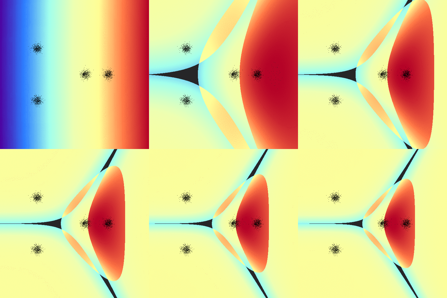
Running Softmax regression slowly on some easy dataset. It's easy to get this to converge in only a handful of iterations.

Of course we can break this naiive implementation. These are some of the nicest behaved gaussians I’ve ever seen. Additionally, I haven’t put any of the clusters “behind” another; because of the linear nature of our parameter weights we can’t make nice curves and circles around classes that would potentially allow us to classify the following set. There’s also no constant parameter weight, that may allow us to get past this issue:

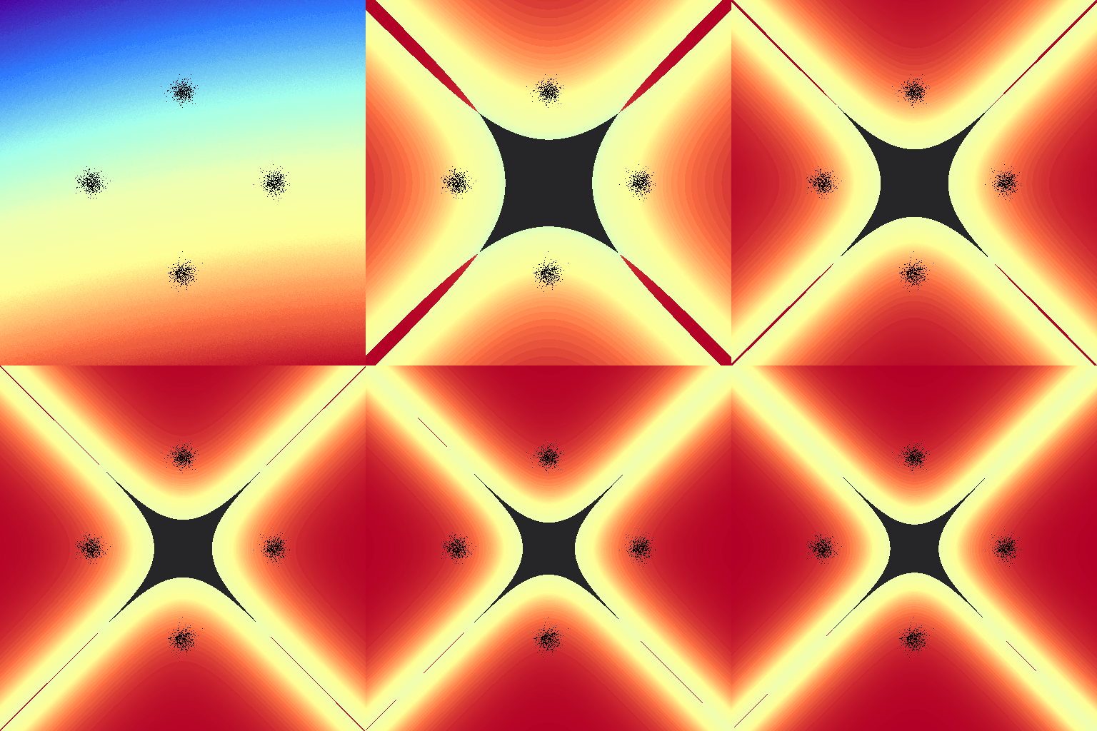
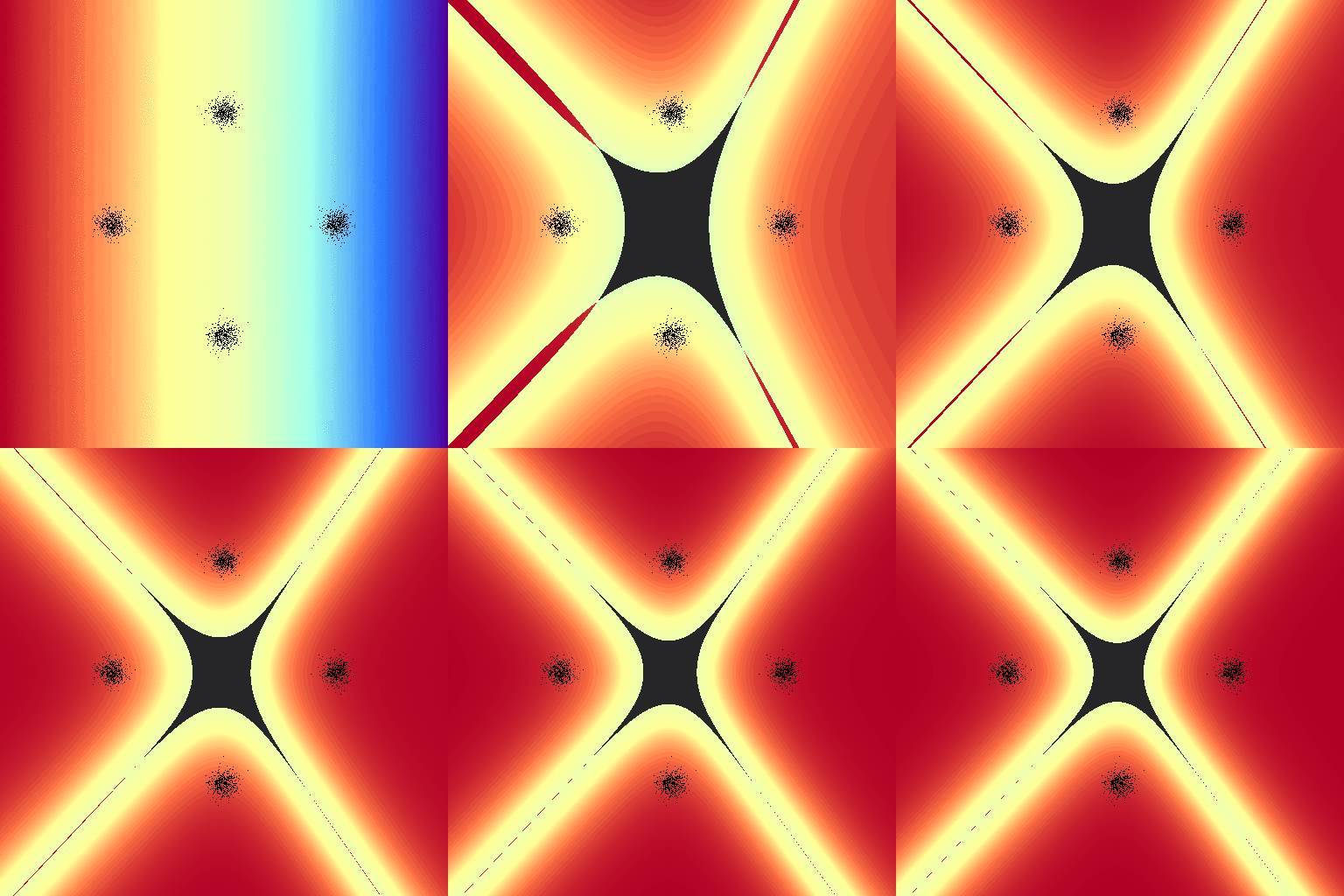
Softmax getting stuck. Also, the grey dots floating around are just a rezult of my colormap screwing up as a result of overlapping probabilities.

On the other hand, this implementation doesn’t suffer the same issue that log-regression did; the exact “line” drawn between classes tends to relax towards a common configuration regardless of the “learning” rates $\alpha$:

With weights which are scewed for one class

References

A general introduction to the exponential family, I believe this was extra material provided as a part of a course taught at Berkely, it was very helpful in expanding upon Ng’s introduction.
Andrew Ng’s lecture on generalized linear models, in which he introduces Softmax Regression.
The Softmax code discussed here is on my Github