Logistic Regression

Motivation

Logistic Regression is the first classification algorithm i’ve come across. It seems somewhat important so I figured it deserved an implementation such that I really “got it”. It also turns out to be a special case of Softmax Regression, a more general classifier which I also intend on implementing. As I think will be typical of these projects, the post and code should be quite short, there’s nothing fancy going on.

The Algorithm

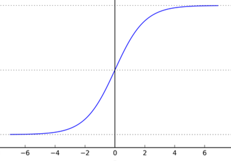
Where least squares regression attempts to find a line that fits data, logistic regression attempts to find a line that divides two classes of data. In fact it doesn’t do this with a line at all, but by fitting a logistic function (now our hypothesis function, $h$) to the data:

$$ h_{\theta}(x) = \frac{1}{1 + e^{-\theta^Tx}}$$

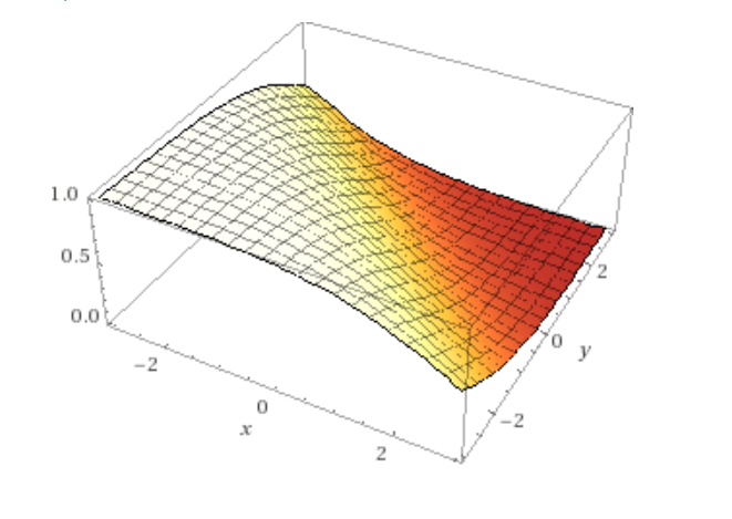
Where the vector $\theta$ contains a weight for every feature (basis vector) of the data. What this looks like as you move up in dimensionality is a division between two regions where the function is high (approaching 1) and low (approaching 0) with a smooth transition between the states. You would interpret the value of the function as the probability of the point being of that class.

The hypothesis sigmoid in one and two dimensions, I'll let you imagine more

Typically another change is made. The regression is made such that the log likelihood of the parameters $\theta$ is maximized. Whereas before, the error given the data and parameters was minimized. Honestly in this case the numbers make more sense than the words for me. Starting off by defining likelihood:

$$ \begin{align}L(\theta) & \equiv P(\vec{y} | x;\theta) \\ &= \prod_{i=1}^mP(y^i | x^i;\theta) \end{align} $$

Which you would read “Likelihood of a set of weights $\theta$ is the probability of seeing the values (classes, $\vec{y}$) given the data points $x$ as parameterized by $\theta$”. And in our case, we mean parameterized by $\theta$ in the logistic function above, though in general it could be parameterized by any function. The second line has broken out of the vector form; products are used when considering joint probability, and here we are considering the joint probability of many points being of a certain class. For the logistic hypothesis function the probability of a point being of a certain class is split into two cases and can be combined with a powers trick:

$$ P(y=1 | x;\theta) = h_{\theta}(x) \\ P(y=0 | x;\theta) = 1 - h_{\theta}(x) \\ P(y | x;\theta) = h_{\theta}(x)^y(1 - h_{\theta}(x))^{1-y} $$

As with least squares regression we want to apply gradient descent, though this time it will be gradient ascent because we are maximizing a function. It is simply a change in sign. As before we want the derivative. Now at this point most people will determine the derivative of the log of the function for likelihood. In general I’ll just say this is to make the required “learning rates” for the algorithm more tractable, as functions aren’t blowing up so much. This is a pretty good response with a little more explanation. Having accepted this, we can then get our derivative:

$$ L(\theta) = \prod_i h_{\theta}(x^i)^{y^i}(1 - h_{\theta}(x^i))^{1-y^i} \\ log(L(\theta)) = \sum_{i=1}^my^ilog(h_{\theta}(x^i) + (1-y^i)log(1-h_{\theta}(x^i))) \\ $$

Letting $h_{\theta}(x_i) \equiv h_i$ to simplify the notation a bit, and splitting the sum before taking a derivative with respect to the j’th parameter weight $\theta_j$:

$$ log(L(\theta)) = \sum_{i, y_i=1}log(h_i) + \sum_{i, y=0}log(1-h_i) \\ \begin{align}\frac{\partial}{\partial\theta_j}log(L(\theta)) & = \sum_{i, y_i=1}\frac{\partial}{\partial\theta_j}log(h_i) + \sum_{i, y=0}\frac{\partial}{\partial\theta_j}log(1-h_i) \\ &= \sum_{i, y_i=1}\frac{1}{h_i}\frac{\partial}{\partial\theta_j}h_i + \sum_{i, y=0}\frac{1}{1-h_i}(-\frac{\partial}{\partial\theta_j}h_i) \end{align} $$

Then sub back in the full form form of the hypothesis function. With $h \equiv \frac{1}{1+E}$, $(1 - h) = \frac{E}{1+E}$ and $E \equiv e^{-\sum_{j=0}^n \theta_jx_j}$.

$$ \begin{align}\frac{\partial}{\partial\theta_j}h & = \frac{-\frac{\partial}{\partial\theta_j}E}{(1+E)^2} \\ &= \frac{-E\frac{\partial}{\partial\theta_j}(-\sum_{j=0}^n\theta_jx_j)}{(1+E)^2} \\ &= \frac{Ex_j}{(1+E)^2} \\ &= h(1-h)x_j \\ \end{align} $$

Then substituting the derivative into each of the split sum terms again, and re-joining the sum terms to get the singular form of the derivative:

$$ \begin{align}log(L(\theta)) & = \sum_{i, y_i = 1}^m(1-h_i)x_{ij} + \sum_{i, y_i=0}^m-h_ix_{ij} \\ &= \sum_{i=0}^my_i - h_{theta}(x_i))x_{ij} \end{align} $$

To maximize the likelihood function then is to add the derivative term with respect to each weight $\theta_j$ and scaled by some factor $\alpha$. You must do this for each feature of your data on every iteration, at least in the naive implementation:

$$ \theta_j := \theta_j + \alpha \sum_{i=0}^m(y_i - h_{\theta}(x_i))x_{ij} $$

And that is exactly the form of the algorithm as it is typically provided. You can also write in gradient notation:

$$ \theta := \theta + \alpha\nabla_{\theta}log(L(\theta)) $$

Code

That was a good bit of proof to read through. Thankfully any implementation will only care about the last line.

def gradientAscent2(x0s, x1s, classes, alphas, weights, index):
	#inner product term for the sigmoid
    res = weights[index]

    dlogLikelyhood = 0

    for i in range(len(classes)): 

	    # update the constant term:	
		if index == 0:
			dlogLikelyhood += alphas[0] * (classes[i] - sigmoid(innerProd2(weights, x0s[i], x1s[i])))
		# update the x0 (x) term:
		elif index == 1:
			dlogLikelyhood += alphas[1] * \
						 (classes[i] - \
	                         	sigmoid(innerProd2(weights, x0s[i], x1s[i]))) * x0s[i]

	    # update the x1 (y) term:
		elif index == 2:
			dlogLikelyhood += alphas[2] * \
						 (classes[i] - \
	                         	sigmoid(innerProd2(weights, x0s[i], x1s[i]))) * x1s[i]

    res += dlogLikelyhood
    return res

This is then called in a loop iterating over the different weights for some number of steps. Obviously its not a robust solution for a data set of any dimensionality.

Results

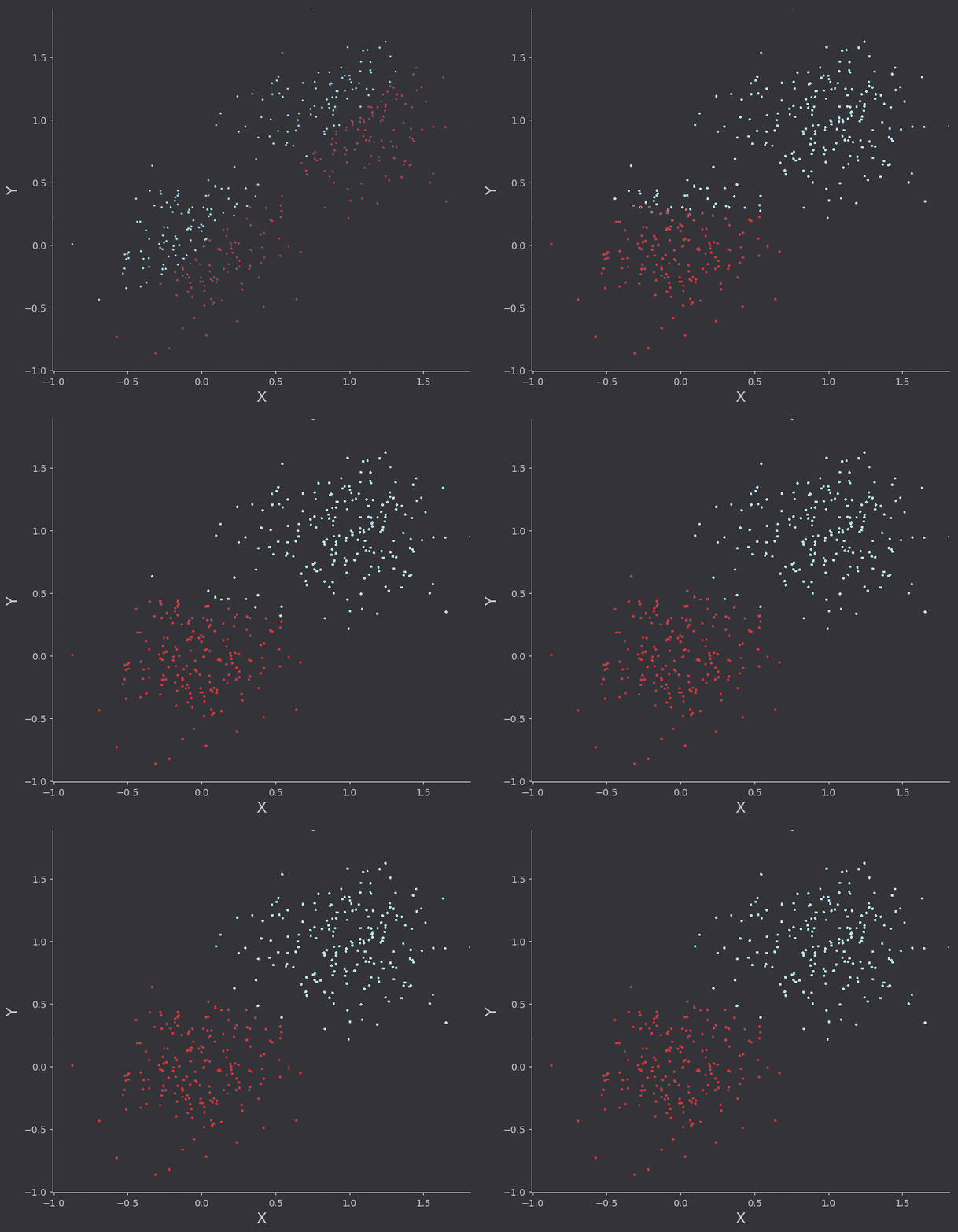
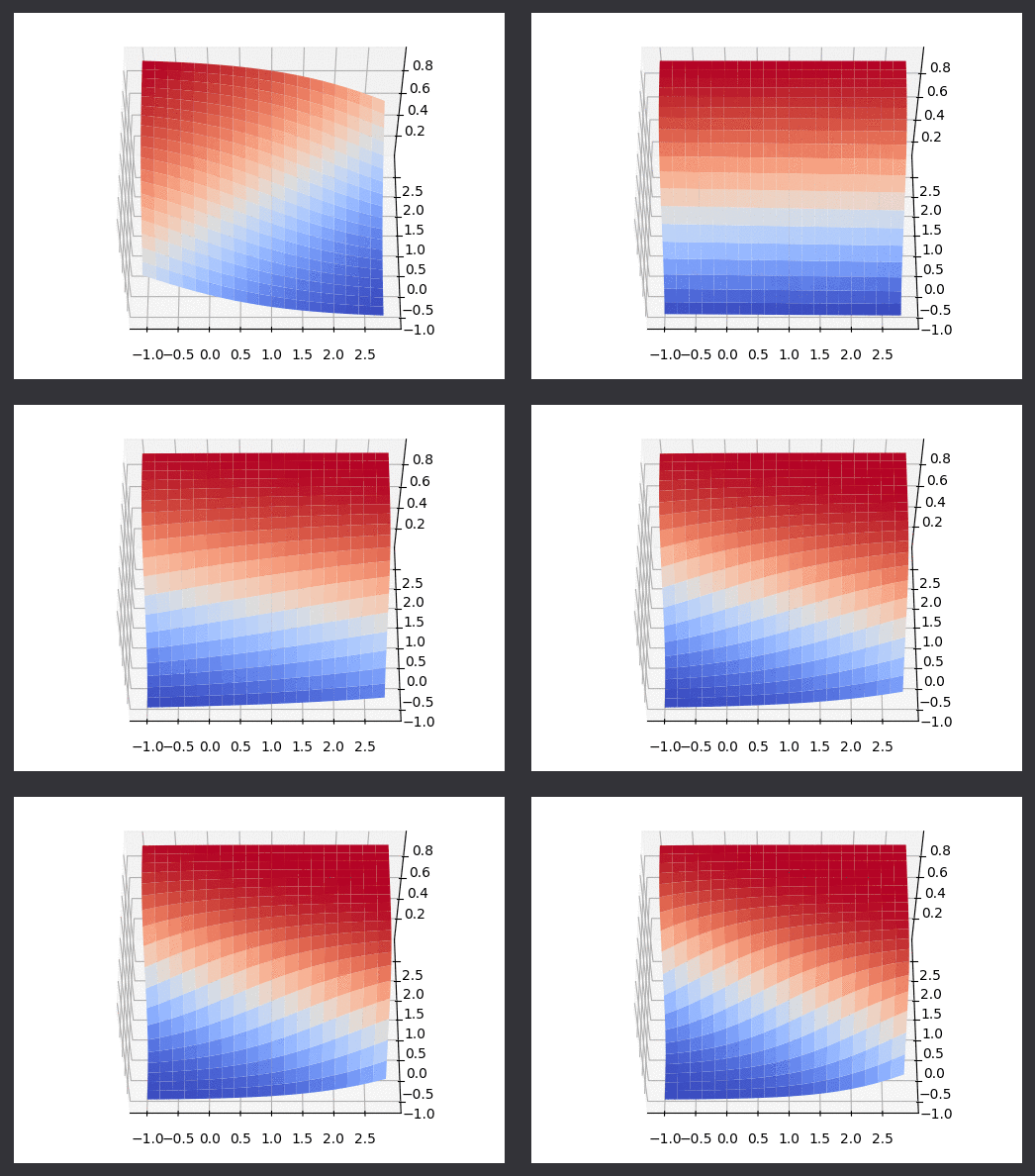
Running with alpha scaling values that are lower than they should be here’s the algorithm in action. I’ve drawn points as they are classified logistic function as it rotates between two gaussian datasets. I’ve also plotted the real logistic surface in a seperate animation.

I was more impressed with the results from this naive implementation than I was with least squares regression. Because the goal is just classification, the choice of alpha parameters was less impactful on the “correct-ness” of the output. It would of course change the number of iterations required, and in this linear case it modifies the final “rotation” of the line with respect to the data. We could of course think of better lines, ones which do not just separate the data into classes, but are also as far as possible from the classes (on average). Thats a task for another time however.

Plotting the sigmoid surface for the same regression run

References

Andrew Ng’s lecture on logistic regression and other topics
Lecture notes on the same subject from a UCSD AI course taught by Charles Elkan.
Code for the regression on My Github. You really could write this one on a napkin though.