Motivation
There are plenty of reasons these days to explore Machine Learning. For me, in reviewing the math behind MCMC methods in a previous project I’d been coming across a lot of people discussing the topic not for Computational Physics applications, but for Machine Learning. A quick look revealed that many of the more advanced topics in Machine Learning share a mathematical foundation with QM (high dimensionality and linear algebra) and at that point I was sold. So in some of the project posts I make from here on out, i’ll be going through freely available lecture resources from Andrew Ng and others and picking out examples to implement.
The Algorithm
A least squares regression algorithm is a means to fit functions to datasets by way of minimizing the error incrementally. For a given input vector $\vec{X}$ you form a guess $h(\vec{X}_i)$ which will have some square error $E_i = (h(\vec{X}_i) - Y_i)^2$
where $i$ just denotes the index of the input vector you are looking at. You can get the total Error by summing over $i$ (that is, summing over all points in your input, using your guess function).
We can then try to minimize the error. We know from basic calc that the minima of a function will be found at a place where its derivative is equal to zero, so set:
Which is described in slightly different notation in Andrew Ng’s lecture, he defines a stand in J(theta) function and finds its derivative specifically for a linear case.
The algorithm is then as follows: chose theta values (which are weights for polynomial terms in your guess, for now at least) and iteratively replace those theta values by
1) subtracting along the direction of the gradient 2) and in proportion to the gradient
Where the gradient is defined in the formula above for one dimension at least. Take enough steps and your function will reach a minimum in error. It doesn’t just “work” however, as you introduce more terms it becomes easy to get stuck in local minima as I will discuss below.
Code
The algorithm is very simple to implement. Most of my time was spent figuring out (again) how to get matplotlib and pyplot to do what I wanted. There was also some pre-processing which needed to be done; the data sets I found to play with, some Chinese weather data provided by UC Irvine, had a few negatives / nulls which needed to be interpolated. Additionally, I found it quite helpful when tuning alpha values to normalize target data sets.
Here’s the algorithm itself though, after that work has been done. I haven’t bothered to generalize it at all:
def squareError(Weights, InputVectors, TargetVector):

	err = 0.0
	for weightSet in range(len(Weights)):
		tempGuess = 0.0
		for idx in range(len(InputVectors[0])):
			tempGuess = Weights[0] * InputVectors[0][idx] #h_theta(X) from Andrew's lecture
			err += (tempGuess - TargetVector[idx]) ** 2

	return err

		# Performing sum of derivs for each order of polynomial asked for
		# Higher order polys get more derivatives and terms added to all weightDerivatives

def firstOrderPolyErrors(weightIdx, vectorIdx, Weights, InputVectors, TargetVector):
	sumOfDerivativeErrors = 0
	if weightIdx == 0:
		sumOfDerivativeErrors += ((Weights[0] + Weights[1] * InputVectors[weightIdx][vectorIdx] - TargetVector[vectorIdx]))
	elif weightIdx == 1:
		sumOfDerivativeErrors += (Weights[0] + Weights[1] * InputVectors[weightIdx][vectorIdx] - TargetVector[vectorIdx]) * InputVectors[weightIdx][vectorIdx]

	return sumOfDerivativeErrors

def batchGradientDescentStep(Weights, InputVectors, TargetVector, Alphas):

	for weightIdx in range(len(Weights)):
		sumOfDerivativeErrors = 0.0
		for idx in range(len(InputVectors[0])):

				# Subtract from the weight the gradient in the associated Input direction
				# whose derivative is equal to the sum [ Err (not squared) * X_i ] where
				# X_i is the InputVector associated with the weight.

			if len(Weights) == 2:
				sumOfDerivativeErrors = tools.firstOrderPolyErrors(weightIdx, idx, Weights, InputVectors, TargetVector)
			elif len(Weights) == 3:
				sumOfDerivativeErrors = tools.secondOrderPolyErrors(weightIdx, idx, Weights, InputVectors, TargetVector)

		Weights[weightIdx] -= Alphas[weightIdx] * sumOfDerivativeErrors

	return Weights
Where the polynomial error functions are just the derivative error function I defined above for specific order polynomials, and I just count the number of weights provided to determine which to use. You can see the rest on my GitHub under the LSR folder.
Results
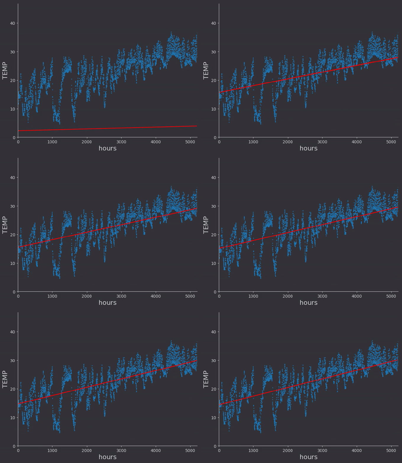
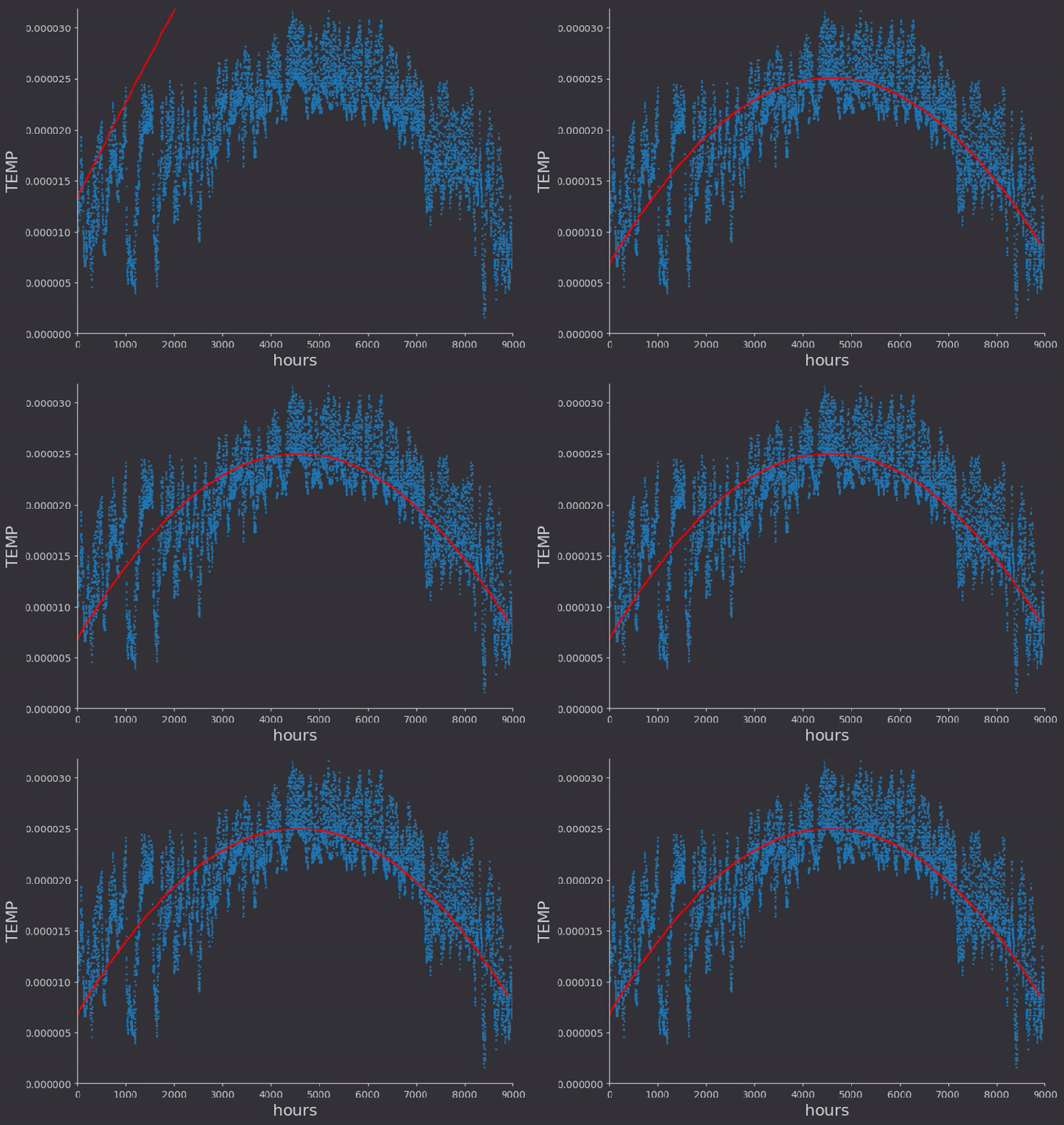
I did a linear fit to a selection of temperature data which had somewhat of a constant run up. Then I expanded the data set to include the winter months, and did a second order polynomial fit to that data.

There were some things which I hadn’t thought of while taking notes from the online lectures. For one, the regression rates for different weights need to be different, very different in fact. In general it seems to me that lower order terms should be ‘learned’ faster than higher order, so that the general location of the proper minima is found. With a quick linear rate for example, the above regression got stuck with a constant offset around zero, as the line quickly found a slope intersecting the data and locking the constant weight from moving, as doing so would increase error (even though there would be a better solution found by doing so)
After working on an MCMC application using randomness and Markov chains with detail balance I know a more probabilistic approach could potentially make quick work of all this alpha parameter tuning, and get rid of the local minima problem entirely. I’ll hold off for now however.

References
I’m cross referencing quite a few resources while I get into this subject, but the core resources are lectures provided online. For this particular post:
-
The first of Andrew Ng’s lectures on Machine Learning, provided by Stanford:
-
Lecture 1: Introduction
-
Lecture 2: linear regression, gradient descent
-
-
The third of Yaser Abu-Mostafa’s lectures, provided by CalTech:
- Lecture 3: The Linear Model
-
Data from UC Irvine’s machine learning repository
-
The code for these regressions on my GitHub in the LSR folder